

R&D LAB Computational Design Shipped Image instrument
Tessera-Mosaic
Image in, paintable sheet out
Any image is broken into flat colour regions, every region gets a number, and out comes a printable vector sheet with a legend, without the image ever leaving the tab.
- 96colours at most, free from 12 up
- 12stages in the chain
- 0,8 slongest compute time on this page
- 0network requests
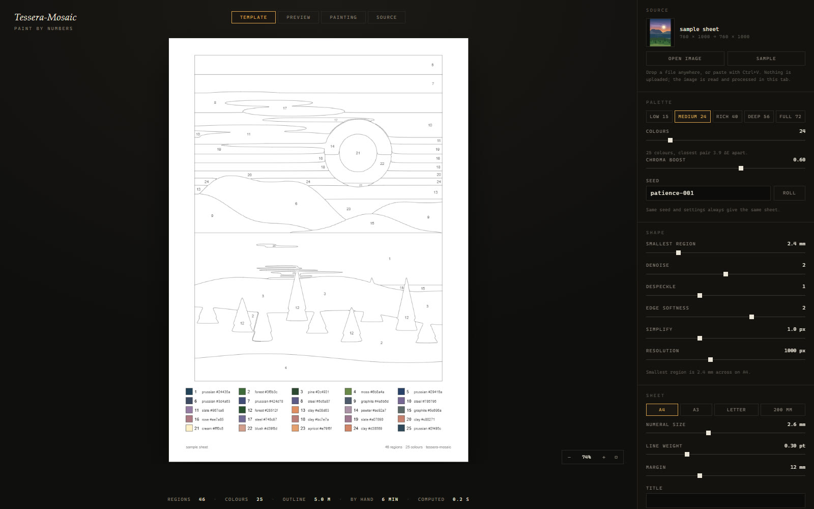
The printable sheet, here on the procedurally drawn sample the application starts with when no file is given: 46 regions, 25 colours. Hairline outlines, a numeral in every region, and under it the legend with swatch, number, nearest colour name, hex value and share of the surface.
Why this is published
The step from an image to something a person actually holds is not a filter, it is a chain of decisions under constraints: segment, merge, simplify, label. Tessera-Mosaic is our evidence that we build such a chain and check it against its own constraints, rather than showing a picture at the end and hoping.
A paint-by-numbers sheet looks like a filter and is not one. A number in a region assumes the region is big enough to paint, not so thin that a brush will not fit, that it has a spot where the numeral fits whole, and that the colour beside it is distinguishable from its neighbours. Tessera-Mosaic is the chain of steps that satisfies those four conditions at once, and three views in which the result can be judged before any paint is bought.
A photograph has no regions
It has gradients, noise and edges that begin nowhere in particular. A painting sheet needs the opposite: closed regions, each big enough for a brush, each in a colour you can buy and find again. Between the two there is no setting, there is a chain.
Four conditions have to hold at once or the sheet is useless. A region needs enough area. It must not be so narrow that no brush fits. It needs a spot where the numeral stands whole. And its colour has to stay distinguishable from its neighbours. Each condition on its own is easy, together they are the problem.
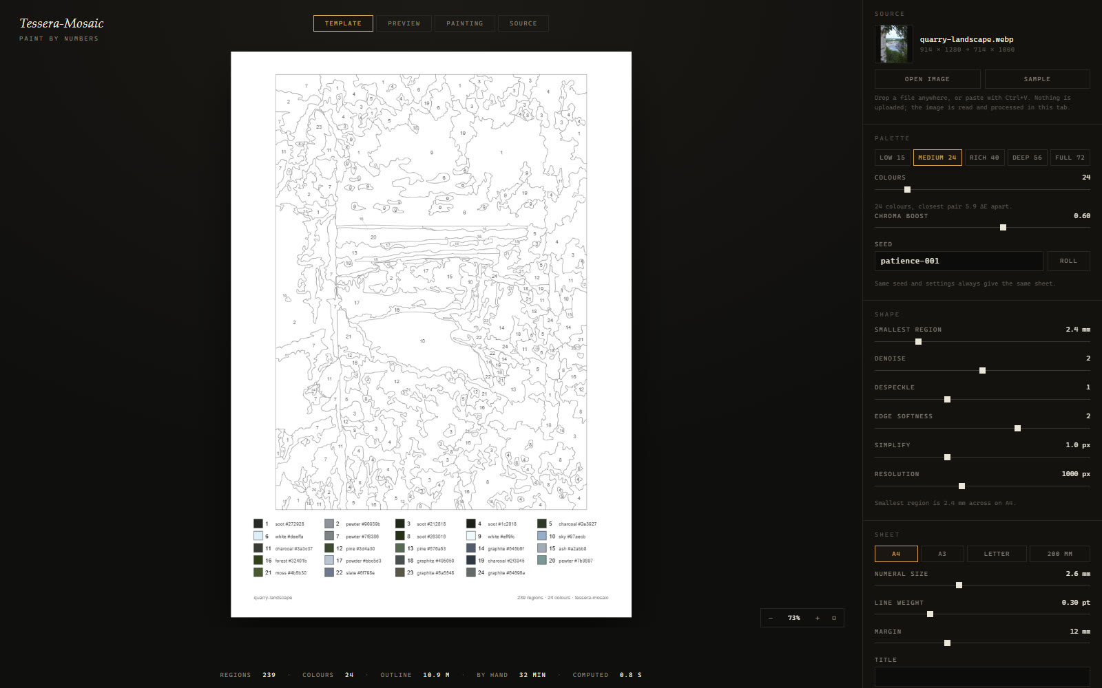
The sheet beside this is computed from a public-domain landscape photograph, 914 x 1280 pixels, dropped to 714 x 1000 working pixels. Out came 239 regions in 24 colours, 10.9 m of outline, 0.8 s of compute. The footer names every one of those numbers before anybody prints.
The whole chain runs in a worker thread
Twelve stages, read as six steps
- 01 Into a colour space where distance means something sRGB goes to CIELAB. Only there does a small distance between two colours also mean that an eye struggles to tell them apart, and only there is the later palette warning a real number rather than a feeling.
- 02 Noise out, edges kept A separable bilateral filter with radius 0 to 4 smooths surfaces and leaves edges standing, so that the next step does not promote grain to a colour of its own.
- 03 Compute the palette Weighted k-means in Lab, k-means++ seeding, 32 Lloyd iterations, and two seeds anchored at the 1st and 99th lightness percentile so that highlight and shadow are not averaged away. Assignment is exact and undithered: a dither here would not be an effect, it would be an unpaintable region.
- 04 Pixels become regions A three by three majority filter votes speckle away, then 4-connected components are labelled. From here on the chain no longer works with colours, it works with areas.
- 05 Merge what is too small or too thin Union-find to fixpoint, with the distance transform re-run between rounds. Too thin is the condition most tools miss: a long narrow band passes every area test and still takes no brush.
- 06 Border, outline, numeral Borders are built as crack edges and chains, each chain smoothed once (Douglas-Peucker, Chaikin, Douglas-Peucker), the outlines assembled, the colours renumbered by painted area, and only then are the numerals placed.
The pipeline builds a mosaic
The one decision
A floating point number decided whether an image was paintable
Three of the five palette tiers did not deliver what their labels said, for a long time. Rich 40, Deep 56 and Full 72 returned a handful of regions and a fraction of the colours asked for, and the more colours were asked for the worse it got. The same sheet that gave 24 colours and 574 regions at Medium came back at Deep with 8 colours and 9 regions.
The cause was one line in the merge. The array holding each region's thickness is a Float32Array, the minimum radius it is tested against is a double. When a region absorbed a neighbour, the thickness of the union was unknown, so the code wrote the minimum radius into it as a claim: this region counts as paintable now. A double stored in a Float32Array is rounded, and about half of all values round down.
When it rounded down, the union was still undersized by its own test. So it absorbed again, and again, until the picture was a few dozen blobs. Which way it rounded depends on the exact value of the minimum radius, and that value is derived from palette size and paper format, so it differs for every combination. The Medium value rounded up and worked. Rich, Deep and Full shared a value that rounded down.
The evidence was uncomfortably clear: a four millionths change in the minimum radius flipped the same sheet between 574 and 79 regions, and comparing the value against its own Float32 rounding predicted which branch you got on twelve of twelve samples.
The decision was then not to repair the comparison but to remove it. The claim now sits beside the region as a flag of its own, the thickness array keeps the honest maximum, and a region that has already merged skips the thinness test. No floating point number decides it any more. Since then every tier delivers its exact palette with no retry at all: Rich 40 with 633 regions, Deep 56 with 618, Full 72 with 874. A sheet from that image now takes 1.0 to 2.2 s instead of 0.6 to 1.0 s, because far more regions survive.
A number meant as a claim was being read back as a measurement.
What 24 colours make of a photograph
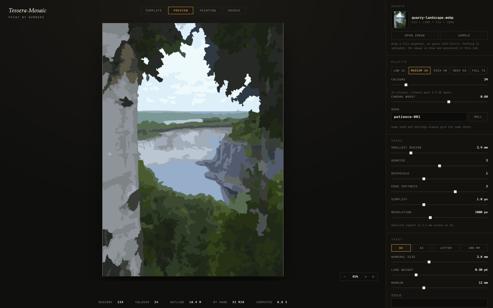
This view exists for one question: is the palette any good, before it is bought. It is the same 239 regions and 24 colours as the sheet further up, only without numerals and without hairlines.
Every palette entry knows its distance to its nearest neighbour. That single number drives the readout under the slider, the shortfall retry, and the refusal when an image cannot carry the colours asked of it. Here 5.9 dE separate the closest pair, and the same photograph also carries all 72 colours, then with 3.7 dE. A flat vector graphic, by contrast, saturates around 50 to 60 colours and says so.
What goes in, what comes out
The photograph
- 914 x 1280 pixels, dropped to 714 x 1000 for the computation.
- Millions of colour values, none of them named.
- Gradients without a border: where the foliage ends is a question of threshold.
- No smallest feature. A branch may be one pixel wide.
- Nothing in it says how long it would take to paint.
The sheet
- 239 closed regions, exactly one numeral in each.
- 24 colours, each with swatch, nearest name, hex value and share of the surface.
- Every region at least 2.4 mm across on A4, or it has been merged away.
- 10.9 m of outline, 0.8 s of compute, an estimated 32 minutes by hand.
- One A4 page as vector, with not a single external reference.
The same frame, two palettes
Fewer colours does not mean fewer regions
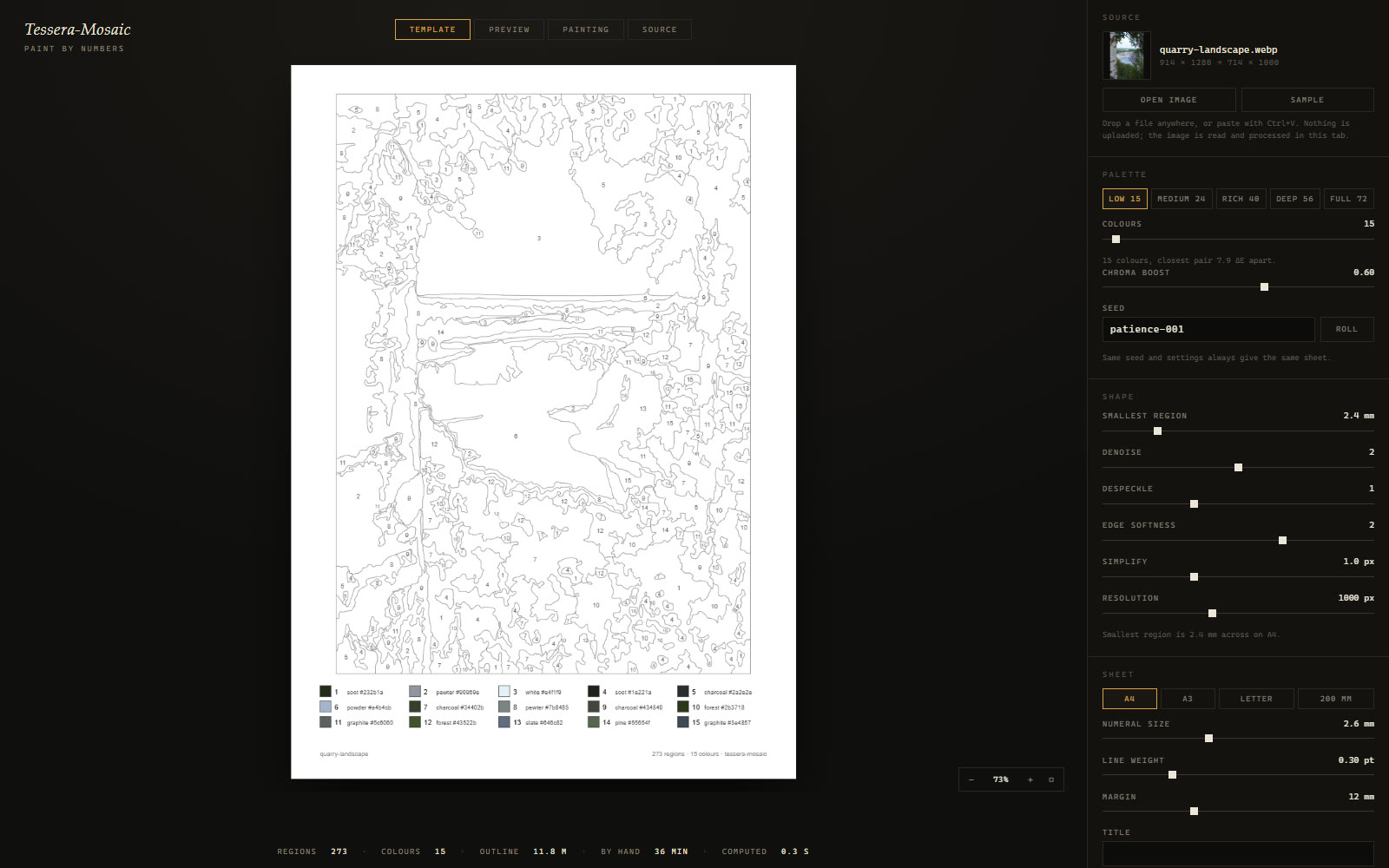
15 colours273 regions, closest pair 7.9 dE, an estimated 36 minutes by hand. That is more regions than at 24 colours, not fewer: a coarse palette frays the border between foliage and sky instead of simplifying it.
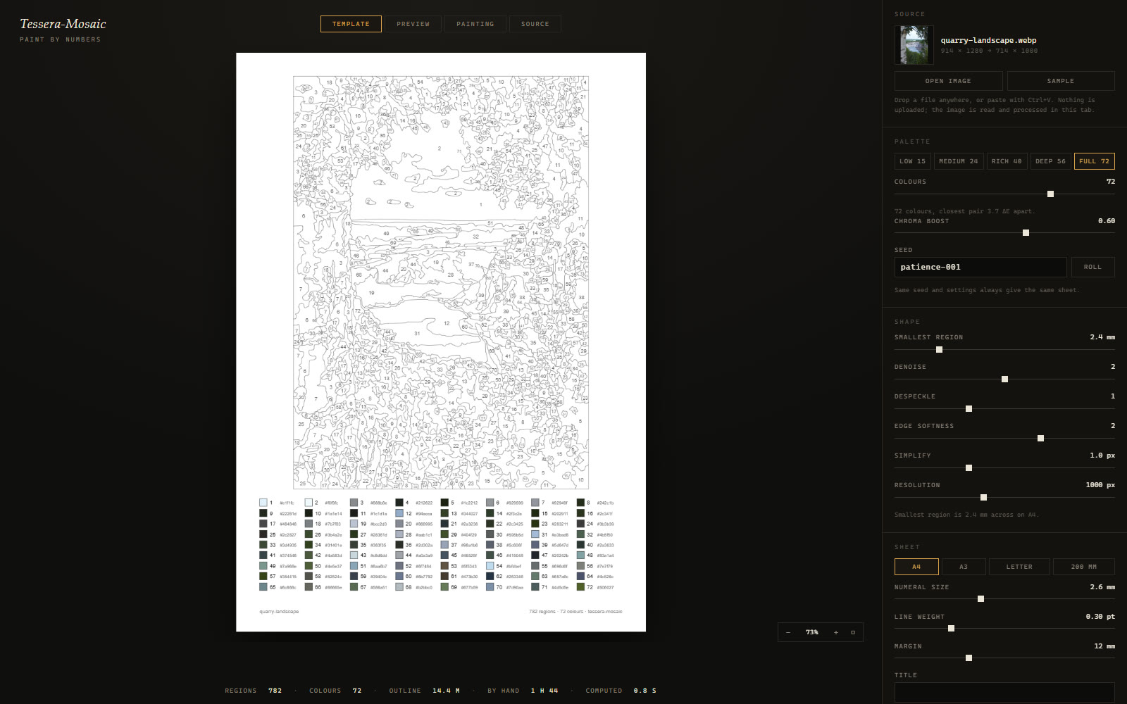
72 colours782 regions, closest pair 3.7 dE, an estimated 1 hour 44 by hand. The photograph carries all 72, and the application says that number instead of hiding it.
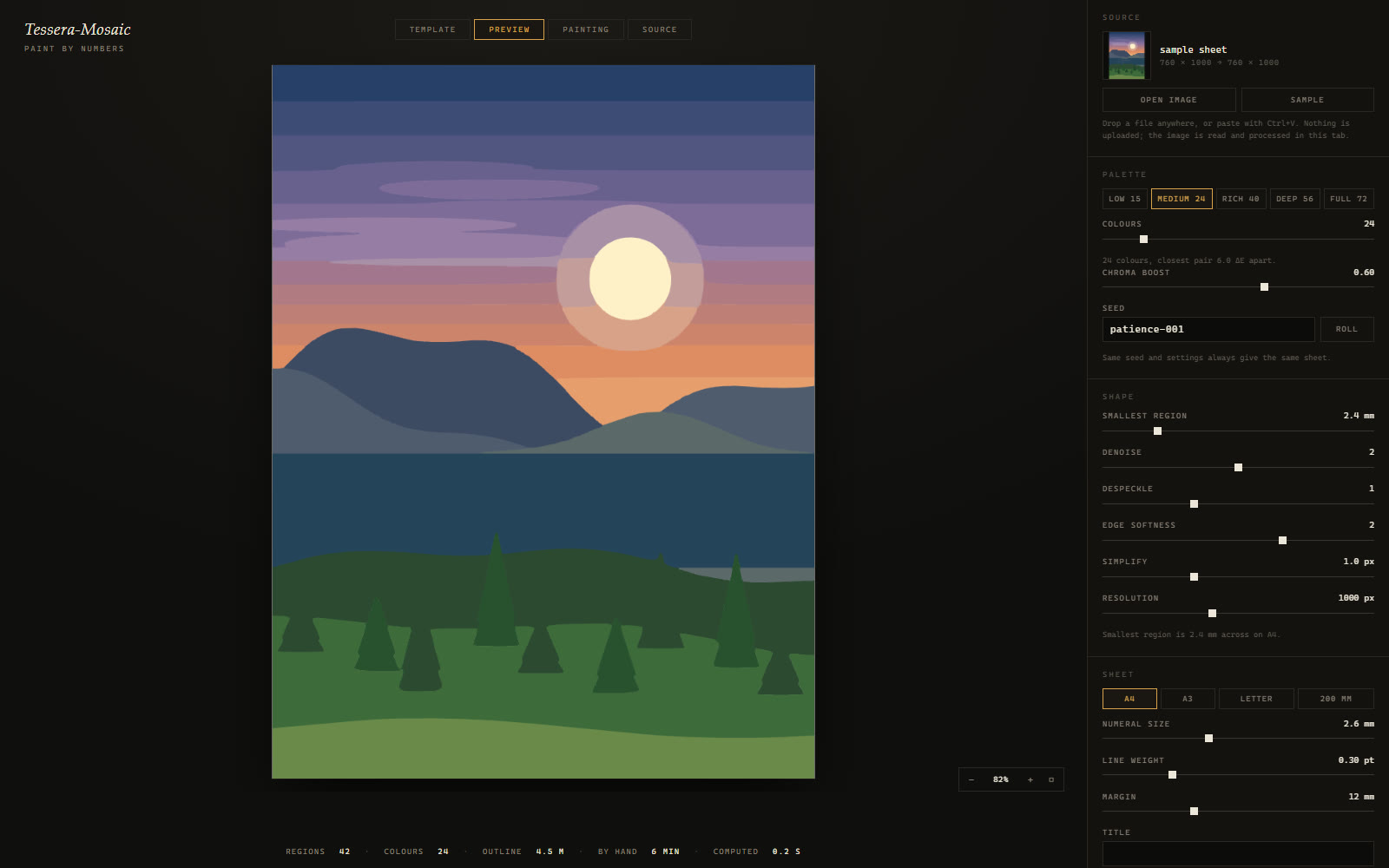
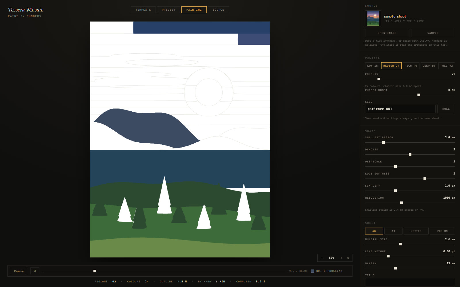
The other two views
Where this fits
- Anything that has to translate an image into something manufacturable: cutting, applique, inlay, tile, vinyl.
- Products where a customer submits their own photograph and expects a physical result that is actually feasible.
- Any problem whose constraint is a minimum size and a minimum width, not only a number of colours.
- Tools that may upload nothing for data protection reasons and still have to run in a browser.
Image credits: every capture shows our own application. Five of them show a result computed from a public-domain photograph: Limestone quarry landscape by Rosendahl, via Wikimedia Commons. The rest use the application's own procedurally drawn sample image.
Why this is published
What this means for your project
More from the lab
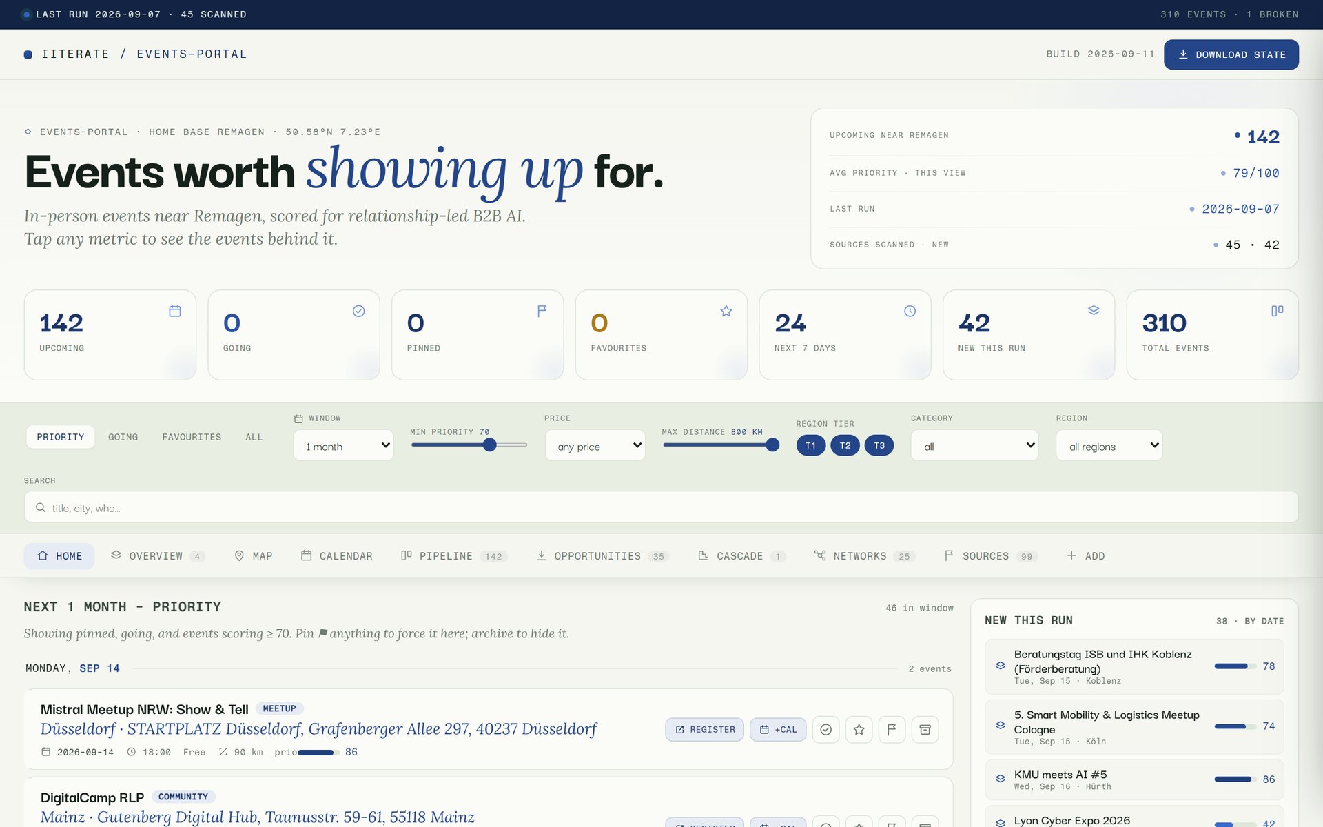 Method Event Scout A language model reads the event pages; everything else is fixed code. What remains is a short list of where a day in person is worth it.
 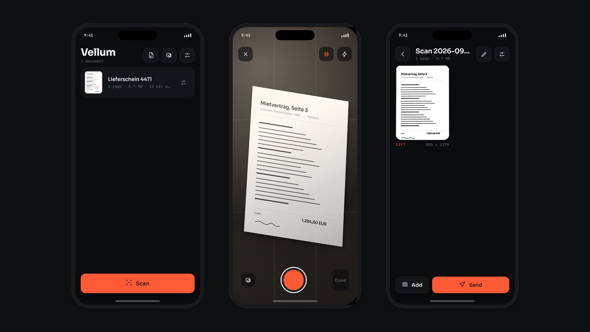 Applied Research Vellum Edges, perspective, light and text are all worked out on the phone. A document leaves the device only when someone sends it.
 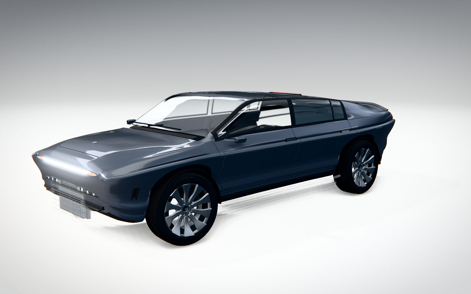 Computational Design Atlas EV1 Twelve chapters take an electric car apart, down to a single cell. No model files, no textures: 327 parts generated from one dimension table.
 Need to turn an image into something manufacturable, under real constraints? That is our kind of problem.
Get in touch